[ MATLAB Tutorial - Lession 5] Operators

An operator is a symbol that tells the compiler to perform specific mathematical or logical manipulations. MATLAB is designed to operate primarily on whole matrices and arrays. Therefore, operators in MATLAB work both on scalar and non-scalar data. MATLAB allows the following types of elementary operations −

• Arithmetic Operators
• Relational Operators
• Logical Operators
• Bitwise Operations
• Set Operations

Arithmetic Operators

MATLAB allows two different types of arithmetic operations −

• Matrix arithmetic operations
• Array arithmetic operations

Matrix arithmetic operations are same as defined in linear algebra. Array operations are executed element by element, both on one-dimensional and multidimensional array.

The matrix operators and array operators are differentiated by the period (.) symbol. However, as the addition and subtraction operation is same for matrices and arrays, the operator is same for both cases. The following table gives brief description of the operators −

Show Examples

Sr.No.	Operator & Description
1	+ Addition or unary plus. A+B adds the values stored in variables A and B. A and B must have the same size, unless one is a scalar. A scalar can be added to a matrix of any size.
2	- Subtraction or unary minus. A-B subtracts the value of B from A. A and B must have the same size, unless one is a scalar. A scalar can be subtracted from a matrix of any size.
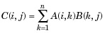
3	* Matrix multiplication. C = A*B is the linear algebraic product of the matrices A and B. More precisely, For non-scalar A and B, the number of columns of A must be equal to the number of rows of B. A scalar can multiply a matrix of any size.
4	.* Array multiplication. A.*B is the element-by-element product of the arrays A and B. A and B must have the same size, unless one of them is a scalar.
5	/ Slash or matrix right division. B/A is roughly the same as B*inv(A). More precisely, B/A = (A'\B')'.
6	./ Array right division. A./B is the matrix with elements A(i,j)/B(i,j). A and B must have the same size, unless one of them is a scalar.
7	\ Backslash or matrix left division. If A is a square matrix, A\B is roughly the same as inv(A)*B, except it is computed in a different way. If A is an n-by-n matrix and B is a column vector with n components, or a matrix with several such columns, then X = A\B is the solution to the equation AX = B. A warning message is displayed if A is badly scaled or nearly singular.
8	.\ Array left division. A.\B is the matrix with elements B(i,j)/A(i,j). A and B must have the same size, unless one of them is a scalar.
9	^ Matrix power. X^p is X to the power p, if p is a scalar. If p is an integer, the power is computed by repeated squaring. If the integer is negative, X is inverted first. For other values of p, the calculation involves eigenvalues and eigenvectors, such that if [V,D] = eig(X), then X^p = V*D.^p/V.
10	.^ Array power. A.^B is the matrix with elements A(i,j) to the B(i,j) power. A and B must have the same size, unless one of them is a scalar.
11	' Matrix transpose. A' is the linear algebraic transpose of A. For complex matrices, this is the complex conjugate transpose.
12	.' Array transpose. A.' is the array transpose of A. For complex matrices, this does not involve conjugation.

Example

The following examples show the use of arithmetic operators on scalar data. Create a script file with the following code −

 Live Demo

a = 10;
b = 20;
c = a + b
d = a - b
e = a * b
f = a / b
g = a \ b
x = 7;
y = 3;
z = x ^ y

When you run the file, it produces the following result −

c =  30
d = -10
e =  200
f =  0.50000
g =  2
z =  343

Functions for Arithmetic Operations

Apart from the above-mentioned arithmetic operators, MATLAB provides the following commands/functions used for similar purpose −

Sr.No.	Function & Description
1	uplus(a) Unary plus; increments by the amount a
2	plus (a,b) Plus; returns a + b
3	uminus(a) Unary minus; decrements by the amount a
4	minus(a, b) Minus; returns a - b
5	times(a, b) Array multiply; returns a.*b
6	mtimes(a, b) Matrix multiplication; returns a* b
7	rdivide(a, b) Right array division; returns a ./ b
8	ldivide(a, b) Left array division; returns a.\ b
9	mrdivide(A, B) Solve systems of linear equations xA = B for x
10	mldivide(A, B) Solve systems of linear equations Ax = B for x
11	power(a, b) Array power; returns a.^b
12	mpower(a, b) Matrix power; returns a ^ b
13	cumprod(A) Cumulative product; returns an array of the same size as the array A containing the cumulative product. If A is a vector, then cumprod(A) returns a vector containing the cumulative product of the elements of A. If A is a matrix, then cumprod(A) returns a matrix containing the cumulative products for each column of A. If A is a multidimensional array, then cumprod(A) acts along the first non-singleton dimension.
14	cumprod(A, dim) Returns the cumulative product along dimension dim.
15	cumsum(A) Cumulative sum; returns an array A containing the cumulative sum. If A is a vector, then cumsum(A) returns a vector containing the cumulative sum of the elements of A. If A is a matrix, then cumsum(A) returns a matrix containing the cumulative sums for each column of A. If A is a multidimensional array, then cumsum(A) acts along the first nonsingleton dimension.
16	cumsum(A, dim) Returns the cumulative sum of the elements along dimension dim.
17	diff(X) Differences and approximate derivatives; calculates differences between adjacent elements of X. If X is a vector, then diff(X) returns a vector, one element shorter than X, of differences between adjacent elements: [X(2)-X(1) X(3)-X(2) ... X(n)-X(n-1)] If X is a matrix, then diff(X) returns a matrix of row differences: [X(2:m,:)-X(1:m-1,:)]
18	diff(X,n) Applies diff recursively n times, resulting in the nth difference.
19	diff(X,n,dim) It is the nth difference function calculated along the dimension specified by scalar dim. If order n equals or exceeds the length of dimension dim, diff returns an empty array.
20	prod(A) Product of array elements; returns the product of the array elements of A. If A is a vector, then prod(A) returns the product of the elements. If A is a nonempty matrix, then prod(A) treats the columns of A as vectors and returns a row vector of the products of each column. If A is an empty 0-by-0 matrix, prod(A) returns 1. If A is a multidimensional array, then prod(A) acts along the first non-singleton dimension and returns an array of products. The size of this dimension reduces to 1 while the sizes of all other dimensions remain the same. The prod function computes and returns B as single if the input, A, is single. For all other numeric and logical data types, prod computes and returns B as double.
21	prod(A,dim) Returns the products along dimension dim. For example, if A is a matrix, prod(A,2) is a column vector containing the products of each row.
22	prod(___,datatype) multiplies in and returns an array in the class specified by datatype.
23	sum(A) Sum of array elements; returns sums along different dimensions of an array. If A is floating point, that is double or single, B is accumulated natively, that is in the same class as A, and B has the same class as A. If A is not floating point, B is accumulated in double and B has class double. If A is a vector, sum(A) returns the sum of the elements. If A is a matrix, sum(A) treats the columns of A as vectors, returning a row vector of the sums of each column. If A is a multidimensional array, sum(A) treats the values along the first non-singleton dimension as vectors, returning an array of row vectors.
24	sum(A,dim) Sums along the dimension of A specified by scalar dim.
25	sum(..., 'double') sum(..., dim,'double') Perform additions in double-precision and return an answer of type double, even if A has data type single or an integer data type. This is the default for integer data types.
26	sum(..., 'native') sum(..., dim,'native') Perform additions in the native data type of A and return an answer of the same data type. This is the default for single and double.
27	ceil(A) Round toward positive infinity; rounds the elements of A to the nearest integers greater than or equal to A.
28	fix(A) Round toward zero
29	floor(A) Round toward negative infinity; rounds the elements of A to the nearest integers less than or equal to A.
30	idivide(a, b) idivide(a, b,'fix') Integer division with rounding option; is the same as a./b except that fractional quotients are rounded toward zero to the nearest integers.
31	idivide(a, b, 'round') Fractional quotients are rounded to the nearest integers.
32	idivide(A, B, 'floor') Fractional quotients are rounded toward negative infinity to the nearest integers.
33	idivide(A, B, 'ceil') Fractional quotients are rounded toward infinity to the nearest integers.
34	mod (X,Y) Modulus after division; returns X - n.*Y where n = floor(X./Y). If Y is not an integer and the quotient X./Y is within round off error of an integer, then n is that integer. The inputs X and Y must be real arrays of the same size, or real scalars (provided Y ~=0). Please note − mod(X,0) is X mod(X,X) is 0 mod(X,Y) for X~=Y and Y~=0 has the same sign as Y
35	rem (X,Y) Remainder after division; returns X - n.*Y where n = fix(X./Y). If Y is not an integer and the quotient X./Y is within roundoff error of an integer, then n is that integer. The inputs X and Y must be real arrays of the same size, or real scalars(provided Y ~=0). Please note that − rem(X,0) is NaN rem(X,X) for X~=0 is 0 rem(X,Y) for X~=Y and Y~=0 has the same sign as X.
36	round(X) Round to nearest integer; rounds the elements of X to the nearest integers. Positive elements with a fractional part of 0.5 round up to the nearest positive integer. Negative elements with a fractional part of -0.5 round down to the nearest negative integer.

Relational Operators

Relational operators can also work on both scalar and non-scalar data. Relational operators for arrays perform element-by-element comparisons between two arrays and return a logical array of the same size, with elements set to logical 1 (true) where the relation is true and elements set to logical 0 (false) where it is not.

The following table shows the relational operators available in MATLAB −

Show Examples

Sr.No.	Operator & Description
1	< Less than
2	<= Less than or equal to
3	> Greater than
4	>= Greater than or equal to
5	== Equal to
6	~= Not equal to

Example

Create a script file and type the following code −

 Live Demo

a = 100;
b = 200;
if (a >= b)
max = a
else
max = b
end

When you run the file, it produces following result −

max =  200

Apart from the above-mentioned relational operators, MATLAB provides the following commands/functions used for the same purpose −

Sr.No.	Function & Description
1	eq(a, b) Tests whether a is equal to b
2	ge(a, b) Tests whether a is greater than or equal to b
3	gt(a, b) Tests whether a is greater than b
4	le(a, b) Tests whether a is less than or equal to b
5	lt(a, b) Tests whether a is less than b
6	ne(a, b) Tests whether a is not equal to b
7	isequal Tests arrays for equality
8	isequaln Tests arrays for equality, treating NaN values as equal

Example

Create a script file and type the following code −

 Live Demo

% comparing two values
a = 100;
b = 200;
if (ge(a,b))
max = a
else
max = b
end

% comparing two different values
a = 340;
b = 520;
if (le(a, b))
   disp(' a is either less than or equal to b')
else
   disp(' a is greater than b')
end

When you run the file, it produces the following result −

max =  200
a is either less than or equal to b

Logical Operators

MATLAB offers two types of logical operators and functions −

• Element-wise − These operators operate on corresponding elements of logical arrays.
• Short-circuit − These operators operate on scalar and, logical expressions.

Element-wise logical operators operate element-by-element on logical arrays. The symbols &, |, and ~ are the logical array operators AND, OR, and NOT.

Short-circuit logical operators allow short-circuiting on logical operations. The symbols && and || are the logical short-circuit operators AND and OR.

Example

Create a script file and type the following code −

 Live Demo

a = 5;
b = 20;
   if ( a && b )
      disp('Line 1 - Condition is true');
   end
   if ( a || b )
      disp('Line 2 - Condition is true');
   end
   
   % lets change the value of  a and b 
   a = 0;
   b = 10;
   
   if ( a && b )
      disp('Line 3 - Condition is true');
   else
      disp('Line 3 - Condition is not true');
   end
   
   if (~(a && b))
   
      disp('Line 4 - Condition is true');
   end

When you run the file, it produces following result −

Line 1 - Condition is true
Line 2 - Condition is true
Line 3 - Condition is not true
Line 4 - Condition is true

Functions for Logical Operations

Apart from the above-mentioned logical operators, MATLAB provides the following commands or functions used for the same purpose −

Sr.No.	Function & Description
1	and(A, B) Finds logical AND of array or scalar inputs; performs a logical AND of all input arrays A, B, etc. and returns an array containing elements set to either logical 1 (true) or logical 0 (false). An element of the output array is set to 1 if all input arrays contain a nonzero element at that same array location. Otherwise, that element is set to 0.
2	not(A) Finds logical NOT of array or scalar input; performs a logical NOT of input array A and returns an array containing elements set to either logical 1 (true) or logical 0 (false). An element of the output array is set to 1 if the input array contains a zero value element at that same array location. Otherwise, that element is set to 0.
3	or(A, B) Finds logical OR of array or scalar inputs; performs a logical OR of all input arrays A, B, etc. and returns an array containing elements set to either logical 1 (true) or logical 0 (false). An element of the output array is set to 1 if any input arrays contain a nonzero element at that same array location. Otherwise, that element is set to 0.
4	xor(A, B) Logical exclusive-OR; performs an exclusive OR operation on the corresponding elements of arrays A and B. The resulting element C(i,j,...) is logical true (1) if A(i,j,...) or B(i,j,...), but not both, is nonzero.
5	all(A) Determine if all array elements of array A are nonzero or true. If A is a vector, all(A) returns logical 1 (true) if all the elements are nonzero and returns logical 0 (false) if one or more elements are zero. If A is a nonempty matrix, all(A) treats the columns of A as vectors, returning a row vector of logical 1's and 0's. If A is an empty 0-by-0 matrix, all(A) returns logical 1 (true). If A is a multidimensional array, all(A) acts along the first non-singleton dimension and returns an array of logical values. The size of this dimension reduces to 1 while the sizes of all other dimensions remain the same.
6	all(A, dim) Tests along the dimension of A specified by scalar dim.
7	any(A) Determine if any array elements are nonzero; tests whether any of the elements along various dimensions of an array is a nonzero number or is logical 1 (true). The any function ignores entries that are NaN (Not a Number). If A is a vector, any(A) returns logical 1 (true) if any of the elements of A is a nonzero number or is logical 1 (true), and returns logical 0 (false) if all the elements are zero. If A is a nonempty matrix, any(A) treats the columns of A as vectors, returning a row vector of logical 1's and 0's. If A is an empty 0-by-0 matrix, any(A) returns logical 0 (false). If A is a multidimensional array, any(A) acts along the first non-singleton dimension and returns an array of logical values. The size of this dimension reduces to 1 while the sizes of all other dimensions remain the same.
8	any(A,dim) Tests along the dimension of A specified by scalar dim.
9	false Logical 0 (false)
10	false(n) is an n-by-n matrix of logical zeros
11	false(m, n) is an m-by-n matrix of logical zeros.
12	false(m, n, p, ...) is an m-by-n-by-p-by-... array of logical zeros.
13	false(size(A)) is an array of logical zeros that is the same size as array A.
14	false(...,'like',p) is an array of logical zeros of the same data type and sparsity as the logical array p.
15	ind = find(X) Find indices and values of nonzero elements; locates all nonzero elements of array X, and returns the linear indices of those elements in a vector. If X is a row vector, then the returned vector is a row vector; otherwise, it returns a column vector. If X contains no nonzero elements or is an empty array, then an empty array is returned.
16	ind = find(X, k) ind = find(X, k, 'first') Returns at most the first k indices corresponding to the nonzero entries of X. k must be a positive integer, but it can be of any numeric data type.
17	ind = find(X, k, 'last') returns at most the last k indices corresponding to the nonzero entries of X.
18	[row,col] = find(X, ...) Returns the row and column indices of the nonzero entries in the matrix X. This syntax is especially useful when working with sparse matrices. If X is an N-dimensional array with N > 2, col contains linear indices for the columns.
19	[row,col,v] = find(X, ...) Returns a column or row vector v of the nonzero entries in X, as well as row and column indices. If X is a logical expression, then v is a logical array. Output v contains the non-zero elements of the logical array obtained by evaluating the expression X.
20	islogical(A) Determine if input is logical array; returns true if A is a logical array and false otherwise. It also returns true if A is an instance of a class that is derived from the logical class.
21	logical(A) Convert numeric values to logical; returns an array that can be used for logical indexing or logical tests.
22	true Logical 1 (true)
23	true(n) is an n-by-n matrix of logical ones.
24	true(m, n) is an m-by-n matrix of logical ones.
25	true(m, n, p, ...) is an m-by-n-by-p-by-... array of logical ones.
26	true(size(A)) is an array of logical ones that is the same size as array A.
27	true(...,'like', p) is an array of logical ones of the same data type and sparsity as the logical array p.

Bitwise Operations

Bitwise operators work on bits and perform bit-by-bit operation. The truth tables for &, |, and ^ are as follows −

p	q	p & q	p | q	p ^ q
0	0	0	0	0
0	1	0	1	1
1	1	1	1	0
1	0	0	1	1

Assume if A = 60; and B = 13; Now in binary format they will be as follows −

A = 0011 1100

B = 0000 1101

-----------------

A&B = 0000 1100

A|B = 0011 1101

A^B = 0011 0001

~A  = 1100 0011

MATLAB provides various functions for bit-wise operations like 'bitwise and', 'bitwise or' and 'bitwise not' operations, shift operation, etc.

The following table shows the commonly used bitwise operations −

Function	Purpose
bitand(a, b)	Bit-wise AND of integers a and b
bitcmp(a)	Bit-wise complement of a
bitget(a,pos)	Get bit at specified position pos, in the integer array a
bitor(a, b)	Bit-wise OR of integers a and b
bitset(a, pos)	Set bit at specific location pos of a
bitshift(a, k)	Returns a shifted to the left by k bits, equivalent to multiplying by 2k. Negative values of k correspond to shifting bits right or dividing by 2|k| and rounding to the nearest integer towards negative infinite. Any overflow bits are truncated.
bitxor(a, b)	Bit-wise XOR of integers a and b
swapbytes	Swap byte ordering

Example

Create a script file and type the following code −

 Live Demo

a = 60;               % 60 = 0011 1100   
b = 13;               % 13 = 0000 1101 
c = bitand(a, b)      % 12 = 0000 1100  
c = bitor(a, b)       % 61 = 0011 1101 
c = bitxor(a, b)      % 49 = 0011 0001 
c = bitshift(a, 2)    % 240 = 1111 0000 */
c = bitshift(a,-2)    % 15 = 0000 1111 */

When you run the file, it displays the following result −

c =  12
c =  61
c =  49
c =  240
c =  15

Set Operations

MATLAB provides various functions for set operations, like union, intersection and testing for set membership, etc.

The following table shows some commonly used set operations −

Sr.No.	Function & Description
1	intersect(A,B) Set intersection of two arrays; returns the values common to both A and B. The values returned are in sorted order.
2	intersect(A,B,'rows') Treats each row of A and each row of B as single entities and returns the rows common to both A and B. The rows of the returned matrix are in sorted order.
3	ismember(A,B) Returns an array the same size as A, containing 1 (true) where the elements of A are found in B. Elsewhere, it returns 0 (false).
4	ismember(A,B,'rows') Treats each row of A and each row of B as single entities and returns a vector containing 1 (true) where the rows of matrix A are also rows of B. Elsewhere, it returns 0 (false).
5	issorted(A) Returns logical 1 (true) if the elements of A are in sorted order and logical 0 (false) otherwise. Input A can be a vector or an N-by-1 or 1-by-N cell array of strings. A is considered to be sorted if Aand the output of sort(A) are equal.
6	issorted(A, 'rows') Returns logical 1 (true) if the rows of two-dimensional matrix A is in sorted order, and logical 0 (false) otherwise. Matrix A is considered to be sorted if A and the output of sortrows(A) are equal.
7	setdiff(A,B) Sets difference of two arrays; returns the values in A that are not in B. The values in the returned array are in sorted order.
8	setdiff(A,B,'rows') Treats each row of A and each row of B as single entities and returns the rows from A that are not in B. The rows of the returned matrix are in sorted order. The 'rows' option does not support cell arrays.
9	setxor Sets exclusive OR of two arrays
10	union Sets union of two arrays
11	unique Unique values in array

Example

Create a script file and type the following code −

 Live Demo

a = [7 23 14 15 9 12 8 24 35]
b = [ 2 5 7 8 14 16 25 35 27]
u = union(a, b)
i = intersect(a, b)
s = setdiff(a, b)

When you run the file, it produces the following result −

a =

    7   23   14   15    9   12    8   24   35

b =

    2    5    7    8   14   16   25   35   27

u =

    2    5    7    8    9   12   14   15   16   23   24   25   27   35

i =

    7    8   14   35

s =

    9   12   15   23   24